The beginner's guide to Excel

Excel makes complex numerical tasks a breeze. All you need is a few formulas, clicks and keystrokes. And voilà – it’s done. Sounds way too good to be true, right?

Mastering Excel’s core functions can be a big help, especially if number crunching is a normal part of your workday. If you want to use Excel like a pro, you’ve come to the right place.

What can I use Excel for?

Excel is incredibly useful for organizing data sets. It’s packed with formulas to help you solve countless numerical problems, manipulate data, and simplify complex calculations. Think of it as a kind of calculator on steroids.

If you still spend many hours manually moving data between cells, rows, and columns in Excel, you need to stop now. Read on to learn the most important Excel shortcuts and make your Excel game as efficient as possible. (Thank us later.)

First steps

• If you’re new to Excel, don’t worry - everyone learns it in different ways. But before you dive in, we recommend brushing up on these basics first.
• Create a spreadsheet from scratch.
• Perform basic calculations within a worksheet, such as: B. Multiply, divide, add and subtract in one worksheet.
• Write and format column titles and text.
• Use the autofill features offered by Excel.
• Add or delete sheets, rows and individual columns. Below we will discuss how you can: B. can add multiple rows and columns.
• Keep row and column titles visible when scrolling through a worksheet. This way you know what data is being inserted as you move further down the document.

If you feel confident about these things, scroll down to get started.

18 important Excel power tips and tricks

1. Pivot tables can be used to understand and make sense of data.
2. Merge multiple columns or rows.
3. Simplify your data by using filters.
4. Remove duplicate records or points.
5. Rows can be transposed into columns.
6. Text can be split between columns.
7. Formulas can be used for basic calculations.
8. Find the average of the numbers in the cells.
9. Conditional formatting can be used to automatically change the color of cells based on the data.
10. The Excel formula IF THEN can be used to automate certain Excel functions.
11. Dollar signs can be used to keep a cell’s formula the same no matter where it moves.
12. The VLOOKUP function can be used to drag data from one part of a worksheet to another part.
13. INDEX COMPARISON formulas can be used to pull data from horizontal columns.
14. The COUNT IF function can be used to make Excel count numbers or words in a range of cells.
15. Use the “&” character to combine cells.
16. Adding checkboxes to a worksheet
17. Link a cell to a website
18. Add dropdown menus

1. Pivot tables can be used to understand and make sense of data

Back to all Excel Power Tips & Ticks

Pivot tables can be used to reorganize data within a spreadsheet. You don’t change your data, but you can compare different information within your spreadsheet and sum values depending on what you want to achieve.

Let’s go through an example together. Let’s say I want to look at the number of employees in each department of GetMyInvoices. You might think that you don’t have a lot of data, but this is very useful for longer data sets.

To create a pivot table, go to Insert > Pivot Table. The pivot table is automatically populated by Excel. However, you can also change the order of the data if you wish. There are four different options you can choose from.

1. Report filter: This option allows you to only view specific rows of your data set. For example, to create a filter by department, you could select only the accounting employees instead of all employees.
2. Column labels: They can be the headings of your record.
3. Line labels: They can be the rows in your dataset. Both column and row labels can contain data from the columns (for example, you can drag the First Name label onto either the column or row label - depending on how you want to see the data).
4. Value: You can use this area to look at the data in a different way. Instead of simply dragging in any numeric value, you can count numbers, use min, max, average, count, sum, or manipulate the data in a number of other ways. By default, when a file is dragged to Value, a count is automatically performed

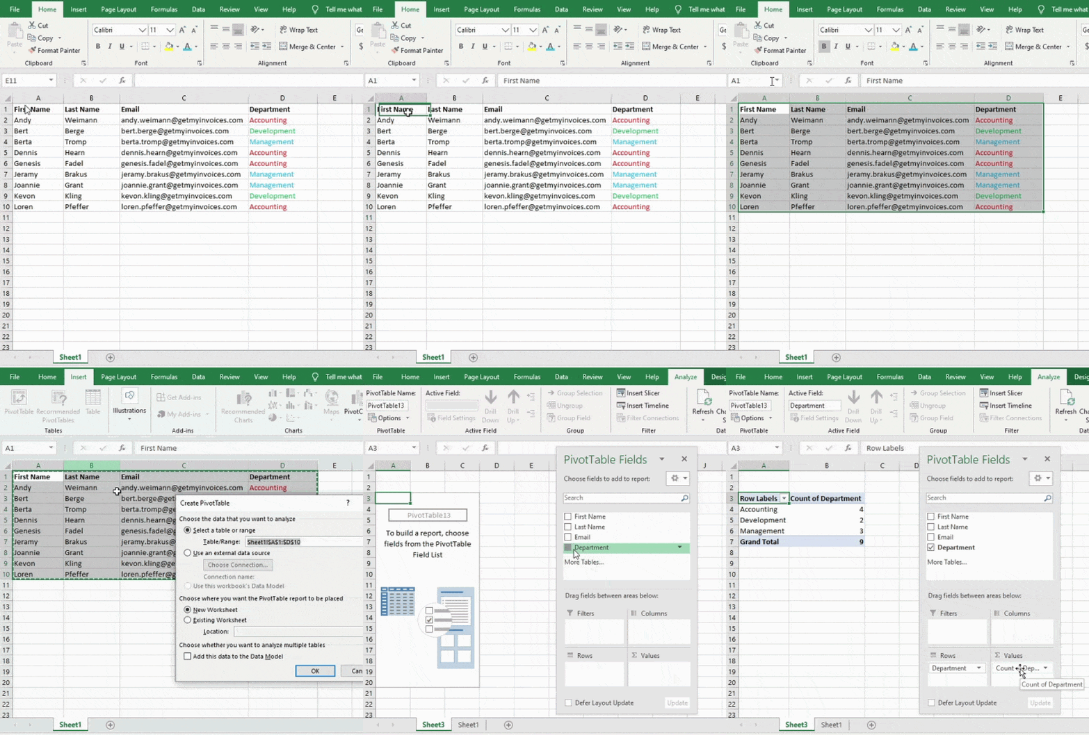
I wanted to count how many employees are in each department, so I go to my pivot table and then drag my department column into both the rows and values. This adds up the number of employees associated with each of the departments.

2. Merge multiple columns or rows.

Back to all Excel Power Tips & Ticks

As you work with your data, you will find that you constantly need to add more columns and rows. Sometimes you may even need to add hundreds of lines. It would be very tedious if you had to do this one by one. Fortunately, Excel offers an easier way to do this.

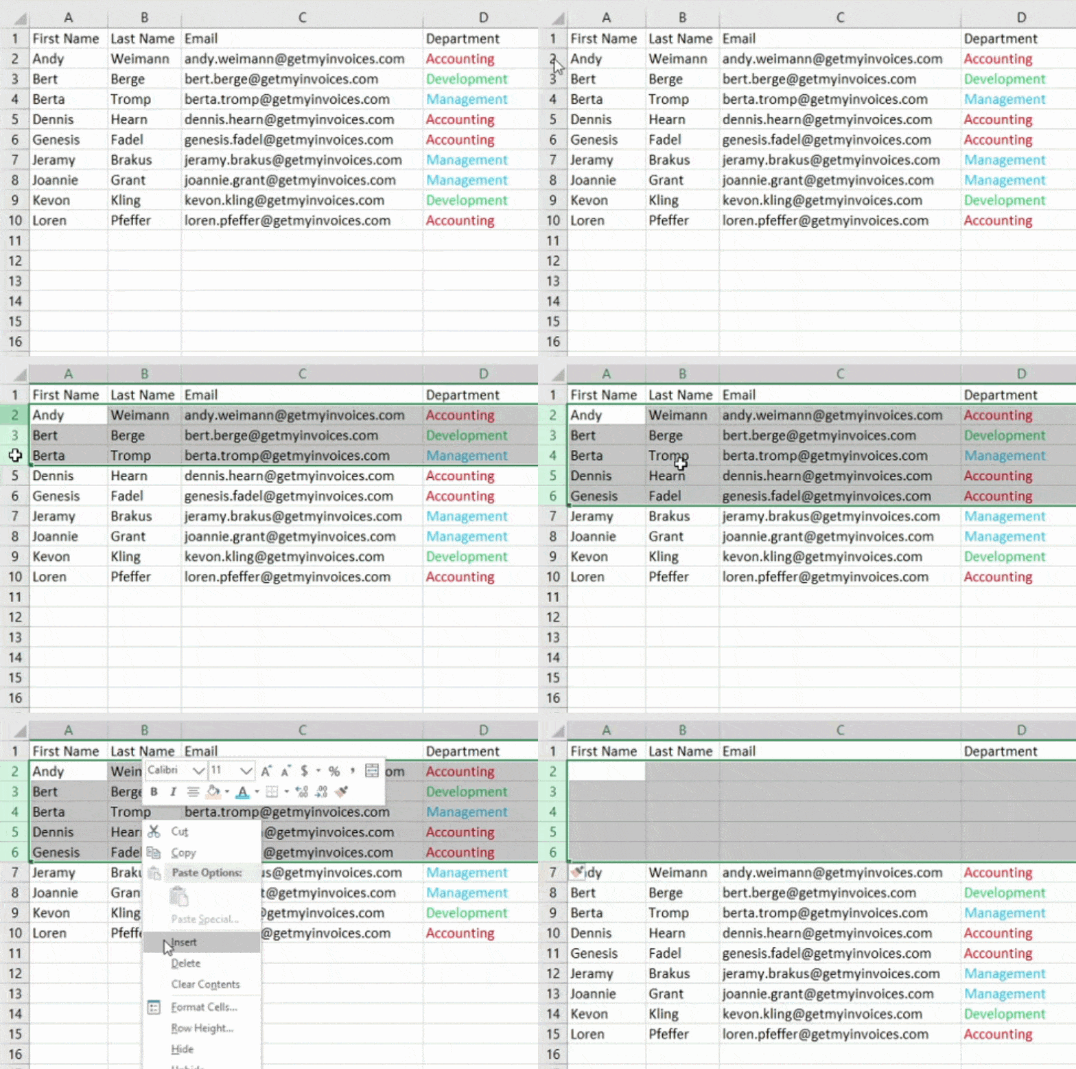
To add more than one column or row in a worksheet, simply select the same number of columns and rows you want to add. Then right-click and select “Paste.”

If you e.g. For example, if you want to add five additional rows, select five rows and click Insert to easily and quickly insert five additional blank rows into your worksheet.

3. Simplify your data by using filters.

Back to all Excel Power Tips & Ticks

When looking through very large data sets, you usually don’t need to look at every single row at once. Sometimes you only want to review data that meets certain criteria. This is where filters can come in handy.

You can use filters to limit your data so that you only view certain rows at a certain time. You can add a filter in Excel for each column that is part of your data. You can then choose which cells you want to view at the same time.

Let’s look at an example. Click the Data tab and then select Filter to add a filter. By clicking the arrow next to the column headings, you can choose whether you want to organize your data in descending or ascending order, or even the specific rows you want to display.

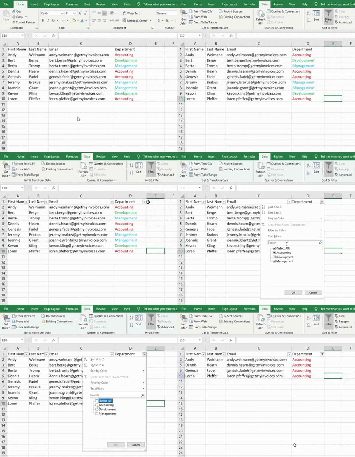
In my example, I only want to see the accounting employees. When I select the “Accounting” filter, the other rows are hidden so I can only focus on the accounting department.

Pro tip: When a filter is enabled, you can copy and paste your values into the worksheet to perform additional analysis in a separate worksheet.

4. Remove duplicate records or points.

Back to all Excel Power Tips & Ticks

There is a tendency for there to be duplicate content in larger data sets. You may have a list of multiple company contacts and just want to see how many companies there are. In such situations, removing the duplicates can be very useful.

To remove duplicates, select the column or row you want to remove duplicates from. Then go to the Data tab and select Remove Duplicates under Tools. A pop-up window will appear asking you to confirm the data you want to work with. Select “Remove Duplicates” and you’re done.

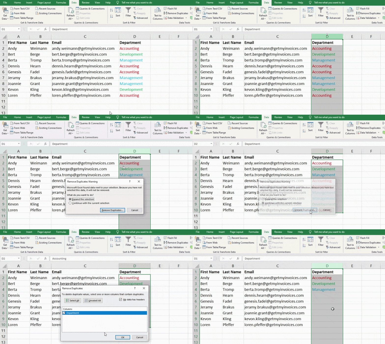
This function can also be used to remove an entire row based on the duplicate column value. If it is e.g. For example, if there are three rows of John Smith information but you only want to view one, you can select the entire record and then duplicates can be removed based on email. The resulting list will only have unique names that contain no duplicates.

5. Rows can be transposed into columns.

Back to all Excel Power Tips & Ticks

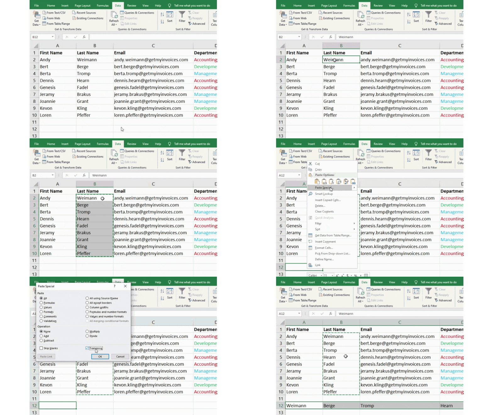
If your spreadsheet has low rows of data, you may want to convert the items from one of the rows to columns (or a column to rows). It would be very time consuming to copy and paste each of these elements into a single header. However, with the transpose feature, you can do this by simply moving your row data to a column or vice versa.

Start by selecting the column you want to transpose into rows. Then right-click it and select Copy. Then select the cells on the worksheet where you want the first column or row to begin. Right-click this cell and then select “Paste Special.” A module will then pop up and you’ll see a transpose option at the bottom. Select the check box and then select OK. This will transfer your column to a row, or vice versa.

6. Text can be split between columns.

Back to all Excel Power Tips & Ticks

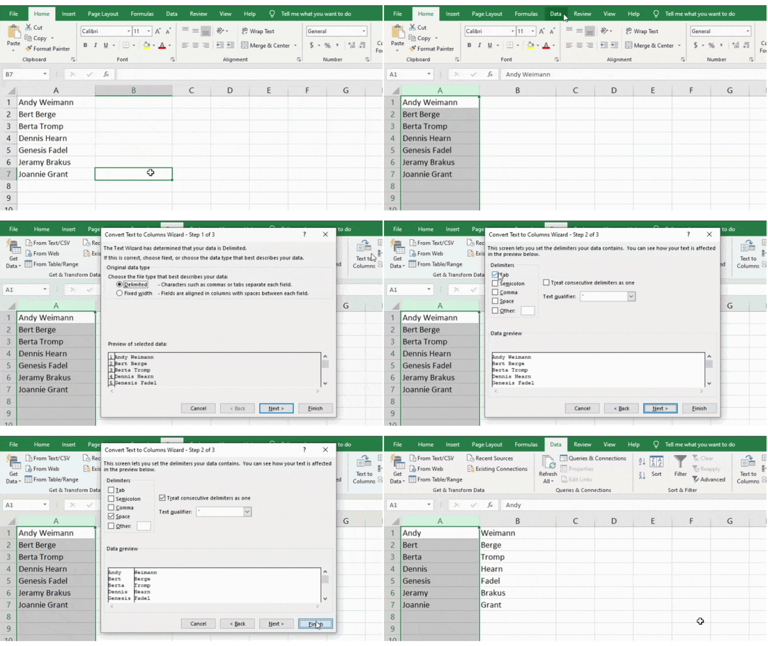
Would you like to be able to split the information contained in a cell into two separate cells? For example, you might want to pull out a company’s name via their email address. Or perhaps you want to split a person’s full name into a first and last name for use in email marketing templates.

Both are possible, thanks to Excel. First select the column you want to split. Then navigate to the Data tab and select Text to Columns. Further information can be found in a module.

First, you need to choose either “Fixed Width” or “Separate”.

• “Fixed width” means that you want to select the exact location where all the columns you want to split should appear.
• “Delimited” means you want to split the column based on characters such as tabs, spaces, or commas.

For our example, let’s choose “Limited” so that the full name can be separated into first and last names.

Now it’s time to choose the limiters. It can be a space, a comma, a semicolon, a tab, or something else (for example, something else can be the “@” sign that an email address uses). We will choose the space character for our example. Excel will then display a preview of what your new columns will look like.

After checking the preview to make sure you’re happy with it, press Next. On this page you can choose “Extended Format” if you wish. Click “Finish” when finished.

Excel formulas

7. Formulas can be used for basic calculations.

Back to all Excel Power Tips & Ticks

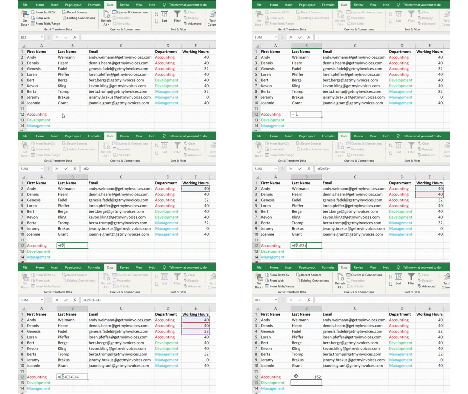
In addition to performing some fairly complex calculations, Excel can also help you with basic arithmetic tasks such as dividing, multiplying, subtracting, or adding your data.

• Use the + sign to add.
• Use the – sign to subtract.
• Use the * sign to multiply.
• Use the / sign to divide

In our example, we will calculate the total number of hours worked by all employees in accounting.

Pro tip: Brackets can also be used to ensure that certain calculations are performed first. In the example (10+10*10), the second and third 10s are multiplied together before the other 10s are added. However, with (10+10)*10, the first two 10s are added first.

8. Find the average of the numbers in the cells.

Back to all Excel Power Tips & Ticks

The formula =AVERAGE(cell range) can be used when you want to have the average for a specific set of numbers. The formula =SUM(cell range) can be used when you want to add a column of numbers.

9. Conditional formatting can be used to automatically change the color of cells based on the data.

Back to all Excel Power Tips & Ticks

You can use conditional formatting to change the color of a cell based on the information contained in the cell. If you e.g. For example, if you want to highlight specific numbers that are in the top 10 % or above average in your worksheet data, this is possible. If you want to color code certain commonalities that different roles have in Excel, that is also possible. This will help you quickly identify important information.

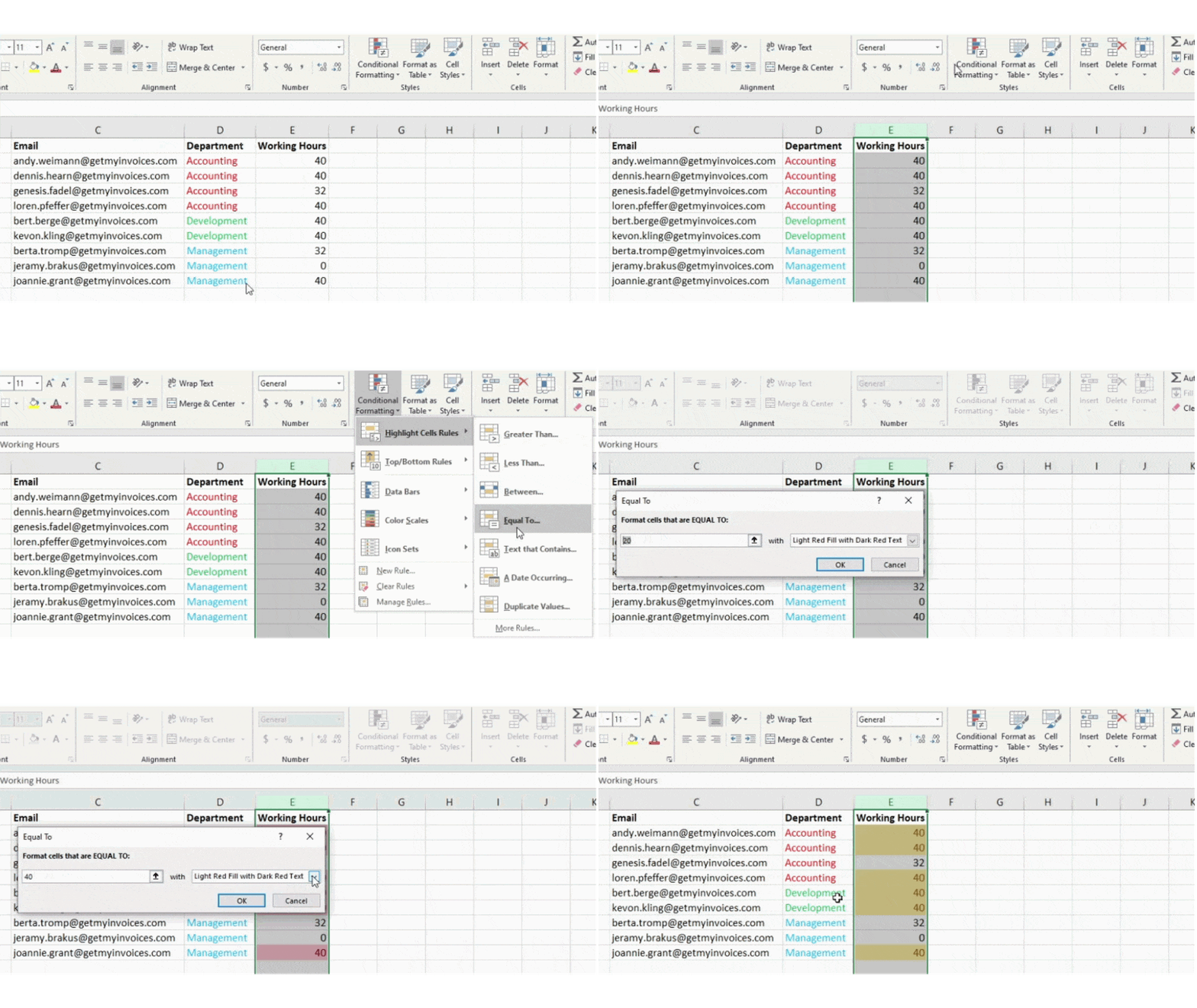
To start the process, select a group of cells that you want to use conditional formatting on. Then select Conditional Formatting from the Home menu and choose your logic from the drop-down menu. (It’s also possible to create your own rule if you want something different). A window will then open asking you to enter more information about your formatting rule. When you’re done, select “OK” and your results will automatically appear.

In our example, we want to highlight in yellow all employees in all departments who have worked 40 hours.

10. The Excel formula IF THEN can be used to automate certain Excel functions.

Back to all Excel Power Tips & Ticks

There are times when you may not want to count the number of times a particular value appears. Instead, you may want to enter other information in a cell if there is a corresponding cell that contains that information.

For example, let’s say I want to give ten points to everyone in accounting. Instead of manually typing a 10 next to each employee’s name from the accounting department, I can instead use the IF-THEN formula to indicate that an employee should receive ten points if they are in the accounting department.

Here is the IF formula: IF(logical_test, value_if_true, valueoffalse)

Our example formula is: =IF(E2=“Accounting”, “YES”, “NO”).

This means that if the employee has 40 working hours, “YES” will automatically be displayed. Otherwise, if the employee has less than 40 working hours, “NO” will automatically be displayed.

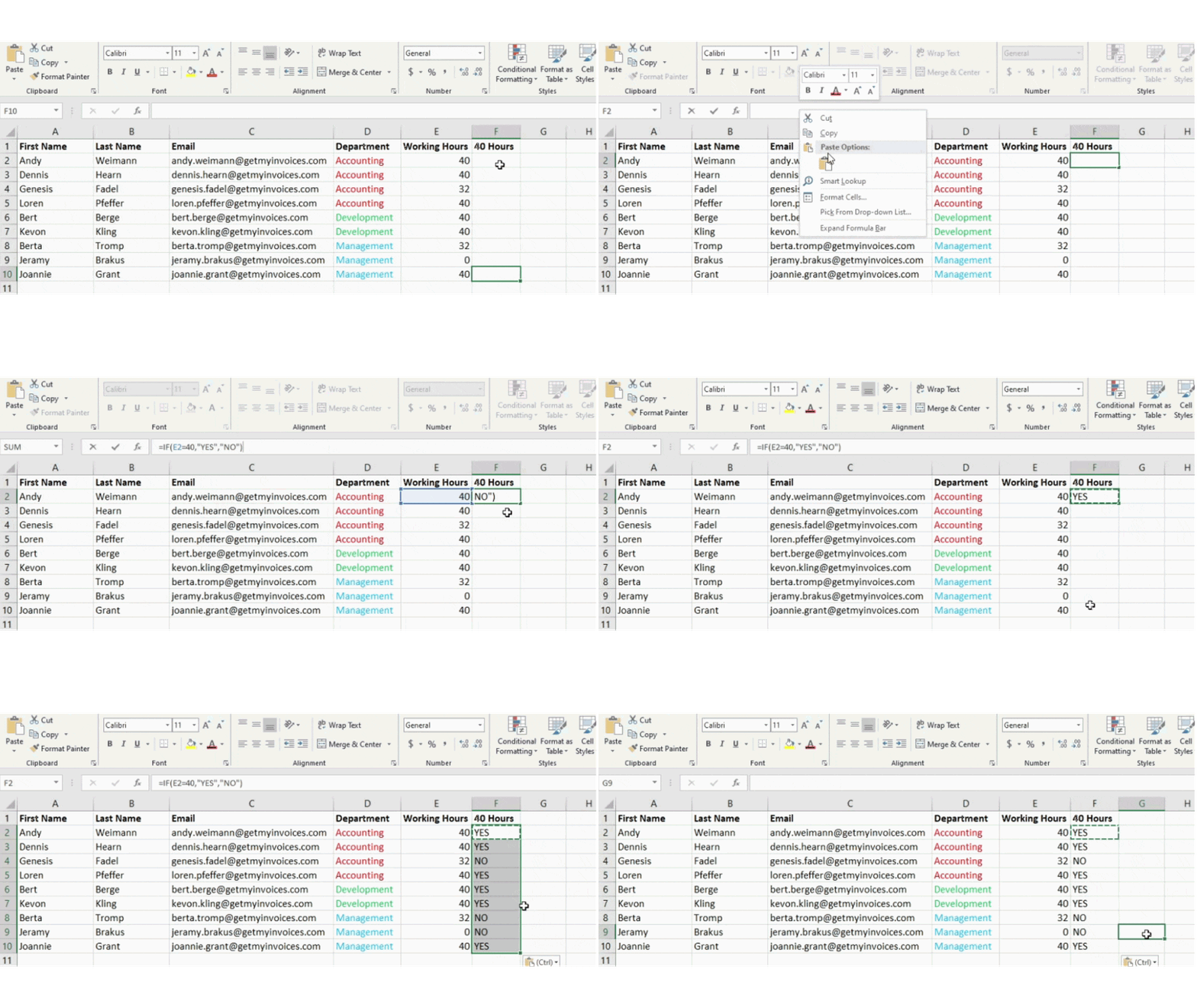
In general, the formula is IF (Logical_Test, Value_if_Correct, Value_if_False). Now let’s take a closer look at the individual variables.

• Logical_Test: The “IF” part of the statement is the logical test. The logic in our example is D2=“Accounting” because we want to ensure that the cell corresponding to the employee contains “Accounting”. Be sure to put “accounting” in quotation marks.
• value_if_true: If the value is true, this should be displayed in the cell. In our example, we want the cell to display “YES” to show that the employee has 40 hours of work. Quotation marks should only be used if you want the result to be displayed in text form and not as a number.
• value_if_false: If the value is wrong, that should be displayed in the cell. For all employees, “NO” should be displayed in the cell to represent less than 40 hours of work. Quotation marks should only be used if you want the result to be displayed in text form and not as a number.

11. Dollar signs can be used to keep a cell’s formula the same no matter where it moves.

Back to all Excel Power Tips & Ticks

Have you ever seen an Excel formula with a dollar sign in it? When the dollar sign is used in a formula, it does not represent the American dollar. Instead, it ensures that the exact row and column are retained even when the same formula is copied to adjacent rows.

A cell reference - if you e.g. E.g. refer from cell C4 to cell A4 – is relative by default. In this case you are referring to a cell five columns to the left (C – A) and also on the same row (4). This is then called a relative formula. When a relative formula is copied from one cell to another cell, it adjusts the values in the formula based on where it is moved. However, sometimes you want these values to remain the same regardless of whether or not they are moved or where they are moved. You can do this by creating an absolute formula in the cell.

To convert the relative formula (=A4+C4) to an absolute formula, we move on to the column and row values with dollar signs, like (=$A$4+$C$4).

Excel functions

12. The VLOOKUP function can be used to drag data from one part of a worksheet to another part.

Back to all Excel Power Tips & Ticks

Do you ever have two sets of data on two different worksheets that you would like to combine into one worksheet?

You could e.g. For example, you might have a list of employee names and their email addresses in one worksheet, with a list of the same employees’ email addresses with their department names in another worksheet - but you would like to have the department names, email addresses, and Have names of people in the same worksheet.

This situation is very common and the best solution is the VLOOKUP function. However, before using the formula, make sure that you have at least one column that is identical in both sheets. Check your data to ensure that the column of data you are using to combine is identical in information and that it does not have any extra spaces.

Here is the formula VLOOKUP(lookup value, table field, column number, [range lookup value])

From our example: = VLOOKUP(C2,Table2!A:B,2,FALSE)

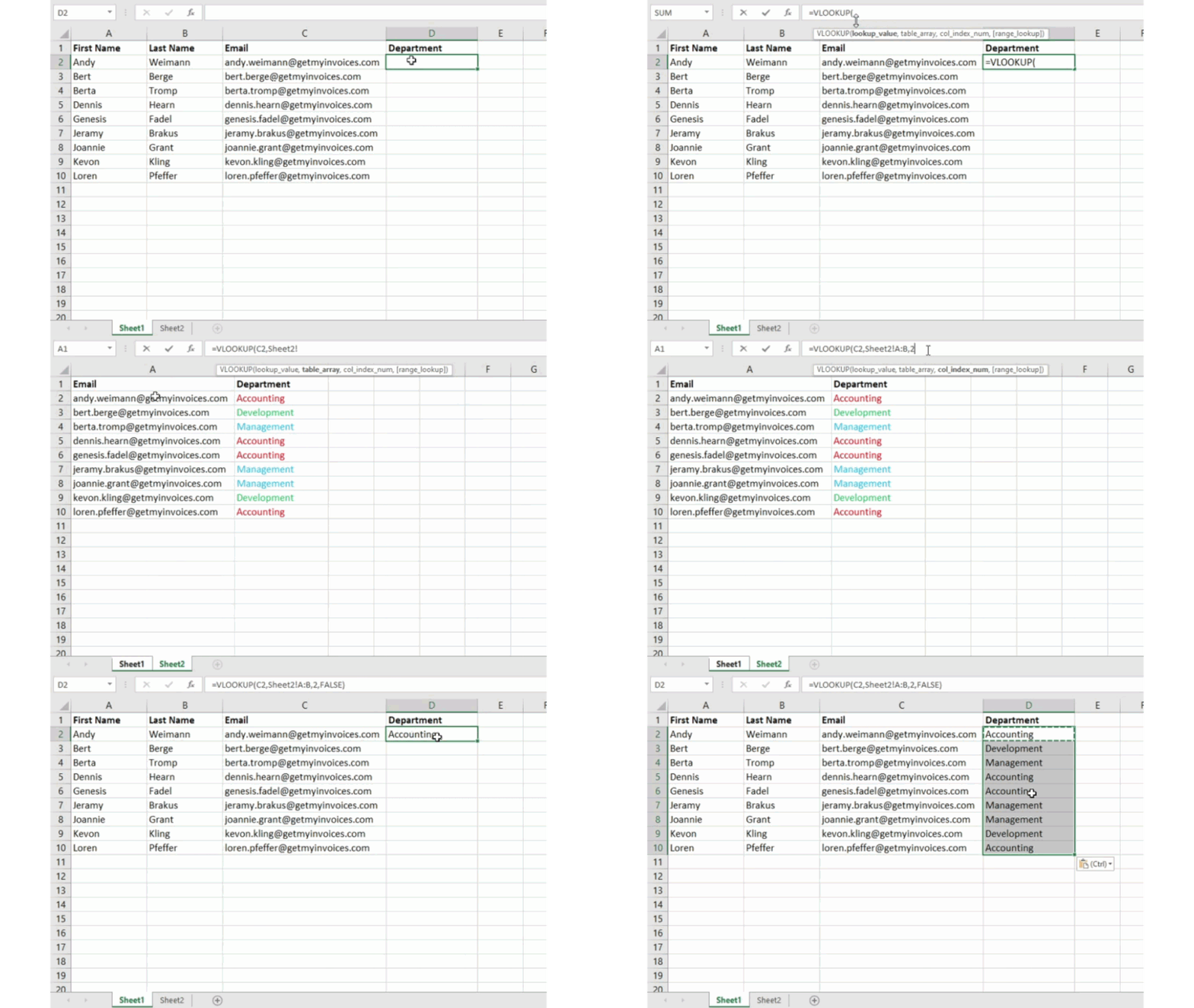
There are several different variables in this formula. If you want to combine information from Table 1 and Table 2 into Table 1, the following applies.

• reference: This refers to the identical value found in both sheets. Select the first value in the first sheet. In our example, this is the first email address in our list, i.e. cell 2 (C2).
• Table array: This refers to the column range on Sheet 2 from which you will pull data, which contains the column with the data identical to the reference (in our example, the email addresses) in Sheet 1, as well as the column with the data you want to copy to sheet 1. In our example this is “Table2!A:B.”, which is column A in Table2. This is the column of Table 2 where our data is identical to the reference (email) found in Table 1. “B” refers to column B, which contains information that only exists in Table 2 and that you want to transfer to Table 1.
• Column number: This is the table field (the column range you specified). It tells Excel which column has your new data that you want to copy to Table 1. In our example, this would be the column in which “Department” is located. In our column range (or table array), “Department” is in the second column, so 2 is the column number. Note: The range can contain more than just two columns. If Table 2 e.g. For example, if you have three columns - Department, Phone Number and Email - you can still refer “Department” to Sheet 1 and VLOOKUP can still be used. The “2” just needs to be changed to a “3” to pull the value into the third column: For example, the result is =VLOOKUP(C2:Table2!A:C,3,FALSE).
• Reference area: FALSE should be used to ensure that you only pull exact value matches.

In our example, Tables 1 and 2 have lists that describe different information about the same people. Their email addresses are the common denominator. Suppose we want to combine these two data sets so that all department information on Table 2 is transferred to Table 1.

If this formula is entered =VLOOKUP(C2,Sheet2!A:B,2,FALSE), all the department’s data will be transferred to Table 1.

Note that VLOOKUP only pulls values from our second table that are to the right of the column that contains the identical data. This can lead to some restrictions. That’s why some people prefer using MATCH and INDEX functions instead.

13. INDEX COMPARISON formulas can be used for pulling data from horizontal columns.

Back to all Excel Power Tips & Ticks

The MATCH and INDEX functions, like VLOOKUP, pull data from another data set to a central location. The main differences are listed below.

• The VLOOKUP-Formula is much simpler. If you are working with large data sets that would require thousands of lookups, you can significantly reduce Excel load time by using the INDEX LOOKUP function.
• One INDEX COMPARISON Formula works from right to left. VLOOKUP formulas, on the other hand, only work as a left-to-right lookup. So if you need to perform a lookup with a lookup column that is to the right of your result column, then you would have to rearrange the columns to perform a VLOOKUP. This can lead to errors or be very tedious if you have large data sets.

So if you want to combine information from Table 1 and Table 2 into Table 1, but Table 1 and 2 do not have the same column values, then to perform a VLOOKUP you would have to switch the columns. In this case, you should do an INDEX COMPARISON instead.

Here is an example. Let’s say Table 1 contains a list of employees’ names along with their GetMyInvoices email addresses, while Table 2 contains a list of employees’ email addresses along with the name of the employee’s manager. The information that is on both tables are the columns that contain the email addresses. However, the email addresses are in different columns on each sheet. I wouldn’t need to switch columns if I used the INDEX MATCH formula instead of VLOOKUP.

So what is the formula? The INDEX COMPARISON formula is the COMPARISON formula nested within the INDEX formula.

Here is the formula: =INDEX(table array, COMPARISON formula)

INDEX COMPARISON: =INDEX(table array, COMPARISON (reference_value, reference_array))

From our example, here is our formula containing the variables: =INDEX(Table2!A:A,(COMPARISON(Table1!C:C,Table2!C:C,0))

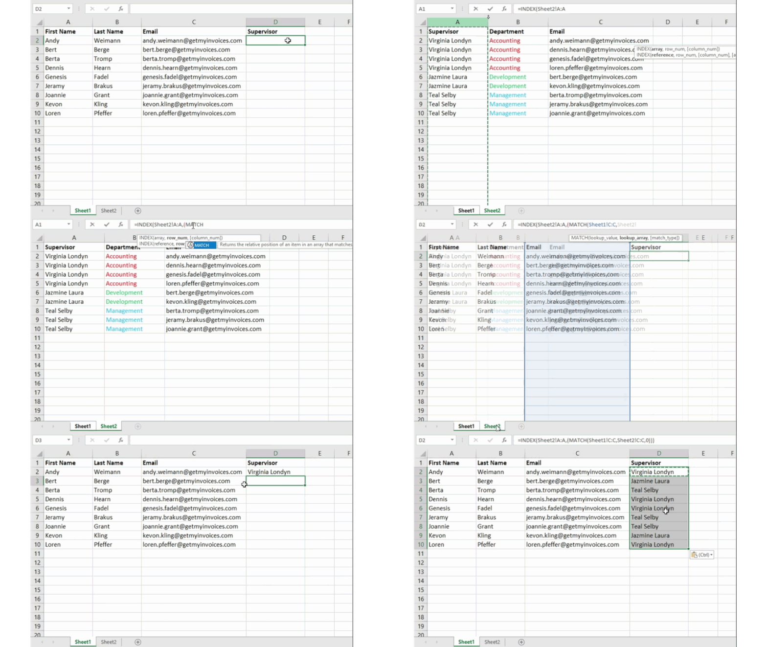
Below are the variables that are used:

– Table array: This is the column range on Table 2 that contains the new data you want to take from Table 1. “A” in our example refers to column A and contains the name of each employee’s manager.

– reference: This refers to the column that is in the table that has identical values present in both sheets. In our example, it is the “Email” column or column C on Table 1, which reads: Table1!C:C.

– Reference array: This column is located on Table 2 and contains the identical values found in both spreadsheets. It refers to the email column in Table 2 in our example, which is also column C: Tablet2!C:C.

After your variables are all correct, enter the formula INDEX MATCH in the top cell of the empty “Supervisor” column on Sheet 1, this is where the combined information should be.

14. The COUNT IF function can be used to make Excel count numbers or words in a range of cells.

Back to all Excel Power Tips & Ticks

Instead of manually counting the number of times a particular number or value occurs, you can let Excel do the work. The COUNTIF function can be used to have Excel count the number of times a number or word appears in a range of cells.

In our example, we would like to count how many times the word “accounting” appears in the data set.

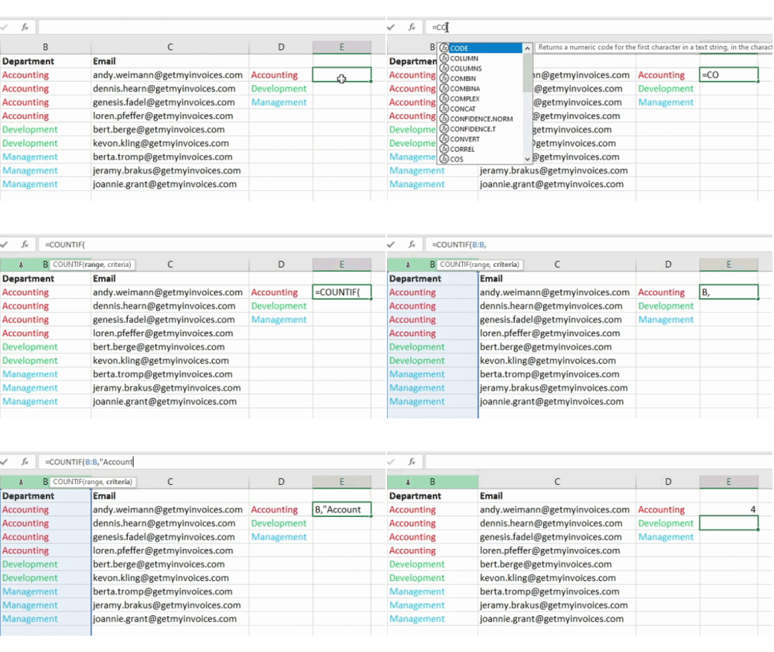
Here is the formula: =COUNTIF(range, criteria)

From our example, here is the formula with variables: =COUNTIF(B:B, “Accounting”)

– Area: This is the range to be covered by the formula. In our case, since we are only focusing on one column, we use “B:B” to indicate that both columns are B.

– criteria: This is any piece of text or number that you want Excel to count. Quotation marks should only be used if you want the result to be in text form and not as a number. The criterion in our example is “accounting”.

Simply enter the COUNTIF formula in any cell and then press Enter to see the number of occurrences of “Accounting” in our data set.

15. Use the “&” character to combine cells.

Back to all Excel Power Tips & Ticks

Databases have a tendency to chunk the data to make it as accurate as possible. So instead of data showing a person’s full name, the database can have data like first and last name in separate columns. Or it could include a person’s location with separate columns for city, state and zip code. You can combine cells with different data into a single cell in Excel by using “&” as a function.

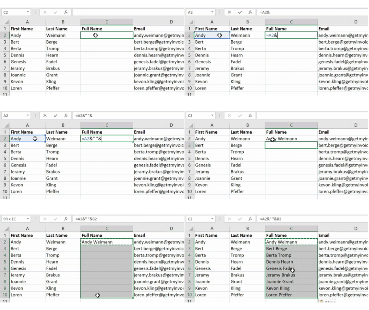
From our example, the formula with variables is: =A2&" “&B2

Let’s go through this formula with an example. Let’s say we want to combine the first and last name as a full name in one column. To do this, place the cursor in the empty cell in which you want the full name. Then select a cell that contains the first name, enter an “&” character, and select the cell that contains the corresponding last name.

If you just type =A2&B2, there will be no space between the person’s first name and last name. Use the =A2&” “&B2 function to add the required space. The quotation marks tell Excel to insert a space between the first name and last name.

To achieve this for multiple rows, simply copy the first cell to other cells using copy/paste.

16. Adding checkboxes to a worksheet

Back to all Excel Power Tips & Ticks

If you’re tracking customer data with an Excel spreadsheet and want to monitor something that isn’t quantifiable, you can add checkboxes in a column.

If you e.g. For example, if you use an Excel spreadsheet to manage prospects and want to track whether or not you called them in the past quarter, you can include a “Called this quarter” column and then check off the cells after you call each customer.

How to add checkboxes in Excel:

Select the cell in your spreadsheet where you want to add check boxes. Then click DEVELOPER. Under SHAPE CONTROLS, click the checkbox.

After the box appears in the cell, copy the box and then select the other cells where you want the box and then paste it.

17. Link a cell to a website

Back to all Excel Power Tips & Ticks

If you use an Excel spreadsheet to track website metrics or social media, you can include a reference column in it that contains links for each row that is in the rack. A URL can be pasted directly into Excel and should be automatically clickable. However, if you use words such as For example, if you need to hyperlink a heading or page title that you are following, follow these steps.

Highlight the words you want to hyperlink. Next, press Shift K. A box will appear where you can enter the URL for the hyperlink. Paste the URL into the field and then click Enter.

If the keyboard shortcut doesn’t work, you can do it manually by selecting the cell and then clicking Insert > Hyperlink

18. Add dropdown menus

Back to all Excel Power Tips & Ticks

You will sometimes use a spreadsheet to track qualitative things like processes. Instead of writing words like “prospect,” “sales lead,” “customer stage,” “yes,” or “no” over and over again in your worksheet, you can instead use drop-down menus to quickly add descriptive characteristics about contacts or other things you to track, to mark.

You can add drop-down menus to cells by doing the following.

Select the cells where you want to have drop-down menus. Then click on the Data menu in the top navigation and press Validation.

A data validation settings box will then open. Under the Allow options, click Lists and then select Drop-down list. Finally, enable the In-Cell Dropdown button and then click OK.

Final thoughts

Now that you’ve learned 18 essential Excel tips and tricks, you’ll be excited the next time you’re dealing with a complex worksheet. If you feel like you need to brush up on your knowledge every now and then, just come back to this article and review a few things you need to move forward.

Excel doesn’t have to intimidate you - learn how to take advantage of its powerful features and you’ll soon appreciate Excel’s sheer capabilities. This guide is designed to help you become a confident, efficient, and productive Excel power user.